1. What Is Financial Macroeconomics? When the Economy Meets the Markets

At the beginning of each month, on a date announced in advance — often, but not always, the first Friday — the U.S. Bureau of Labor Statistics releases its jobs report at 8:30 a.m. New York time. Investors watch the number of payroll jobs created or lost outside agriculture, but also unemployment, wages, working hours, and revisions to previous months (official BLS calendar).

They compare the entire report with the forecasts made before its release — what the market calls the consensus. Automated systems can react within milliseconds; analysts then interpret the details and revisions over the following minutes. Equity-index futures (contracts in which you take a position today on the future level of an index), government-bond yields, and currencies such as the euro or the dollar all adjust, even when the stock exchange itself is not yet open. Stronger-than-expected job creation may, for example, lead investors to anticipate higher interest rates: good economic news is therefore not automatically good news for the stock market.

Nothing has changed yet in the real economy: no factory has produced more, and no household has taken home a bigger paycheck. New information has simply changed the outlook — and with it, the prices investors are willing to pay today. The report itself describes a month that has already ended: what moved was the view of the future, not the past it measures.

This is precisely what financial macroeconomics studies: how growth, inflation, employment, and central banks affect markets, and how markets then feed back into the economy.

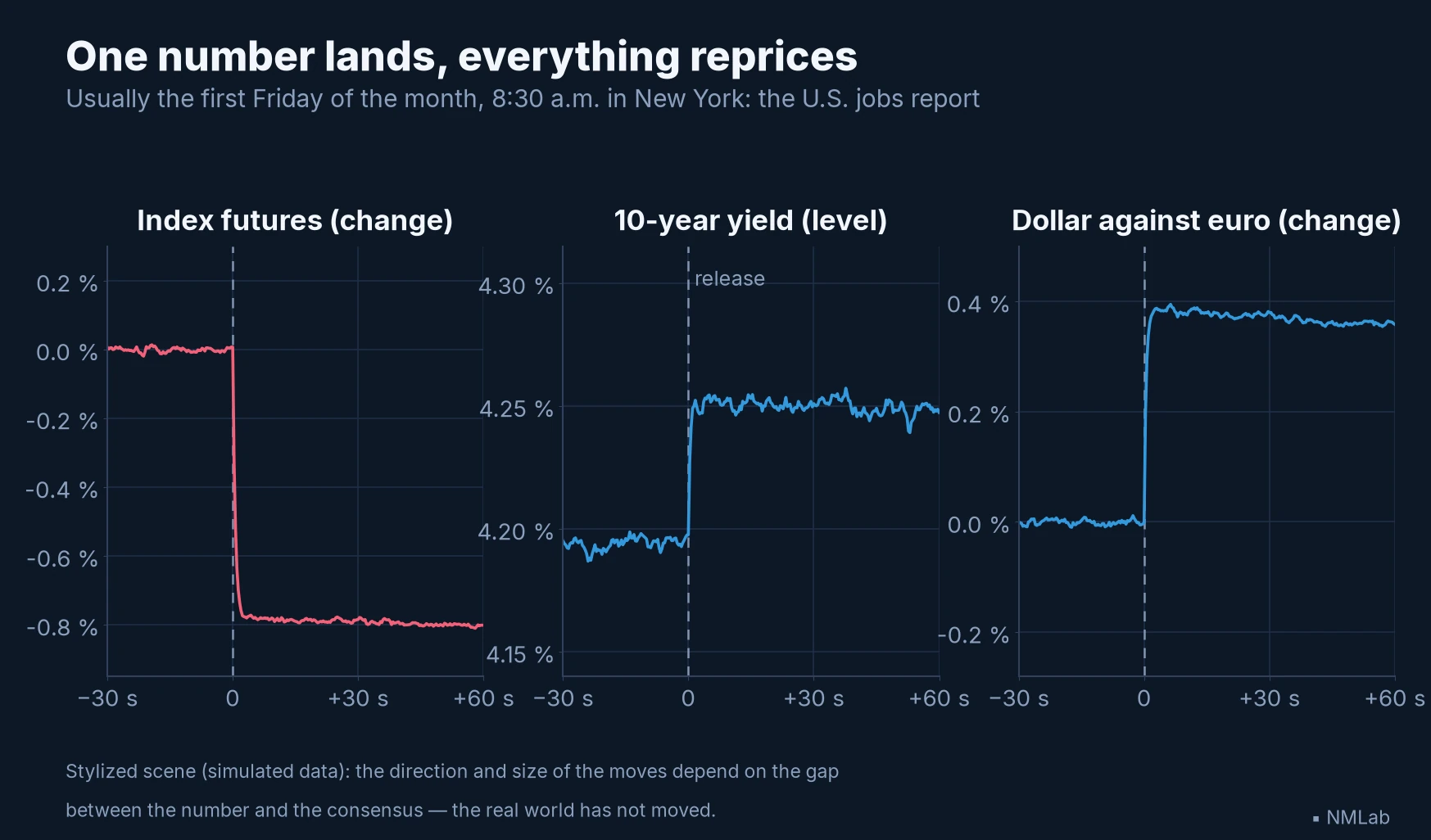
Other reactions are possible: the direction of the move depends on the context, not only on the number.

At a glance — Level: Foundations · Prerequisites: none

By the end of this chapter, you will be able to:

• see what financial macroeconomics connects: an economy that moves slowly, markets that reprice fast;
• explain why markets respond to the expected future rather than to the present;
• trace how growth, inflation and rates reach bonds, equities and currencies;
• understand why what matters about a number is how far it lands from what was expected;
• describe how markets send those movements back into the economy;
• see what this reading makes possible — recognizing a regime, telling a genuine surprise from an expected one — and what it does not.

A few simple formulas show where the quoted figures come from: they are there for the curious, and you can skim them without losing the thread — only the intuition, set in bold, matters for what follows.

The economy on one side, the markets on the other

No one ever built a factory in a single trading session. The real economy — production, income, consumption, investment, employment — moves at the pace of months, quarters, and years; broad indicators such as gross domestic product, inflation, or unemployment sum up the activity of millions of people and businesses.

Financial markets, by contrast, trade almost nothing tangible: mostly, rights to future payments. A stock is a share of ownership in a company: it gives a claim on its assets and profits that ranks after every creditor, and guarantees no payment; a bond is a contractual promise of payments — interest, if any, and repayment — by which a government or a company borrows; a currency — money such as the euro or the dollar — has a value that can only ever be expressed against another currency.

Because every new piece of information can change expected payments, rates and risks, the prices of these rights adjust continuously. Markets allow savers to invest and governments or companies to raise funds, while giving each asset an observable price.

Economic statistics mostly describe activity that has already taken place, whereas a market price tries to value payments that may arrive years from now: the two can move in opposite directions for a while without either one being irrational.

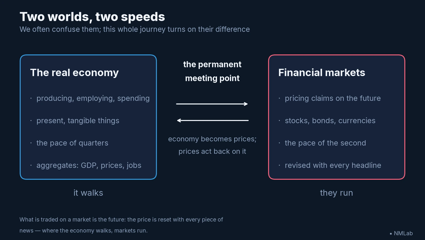
The economy measures what has already happened; markets pay for what might.

A market price is therefore an observable fact, but not a truth about value: it is a collective summary of the available information — what buyers and sellers believe, at that instant, about future payments, interest rates, risks and, for a currency, the relative prospects of the two economies involved. That opinion can be wrong or follow the crowd, but it arrives immediately, while statistics arrive monthly or quarterly.

A bridging discipline

Three different lenses can be trained on the same economy. Microeconomics watches the decisions of a single household or company; macroeconomics takes the economy as a whole — growth, inflation, unemployment, money, and interest rates; corporate financial analysis starts instead from the accounts and prospects of one specific business. For a fuller explanation, see Microeconomics and macroeconomics: the difference.

Financial macroeconomics replaces none of them: it connects them. It studies the common setting — growth, inflation, rates, liquidity (the short-term funding available in the system), and appetite for risk — in which every investment is valued, and it follows that setting in both directions: how the economy and central banks move expected profits, interest rates, and asset prices; then how those prices in turn move credit, consumption, investment, and exchange rates.

Several ideas built this bridge. Keynes stressed the role of expectations in investment; monetarists studied the link between money and inflation; rational expectations described how households and businesses adjust to anticipated policies; and market efficiency examined how prices incorporate information. The common thread is simple: present decisions depend on the expected future.

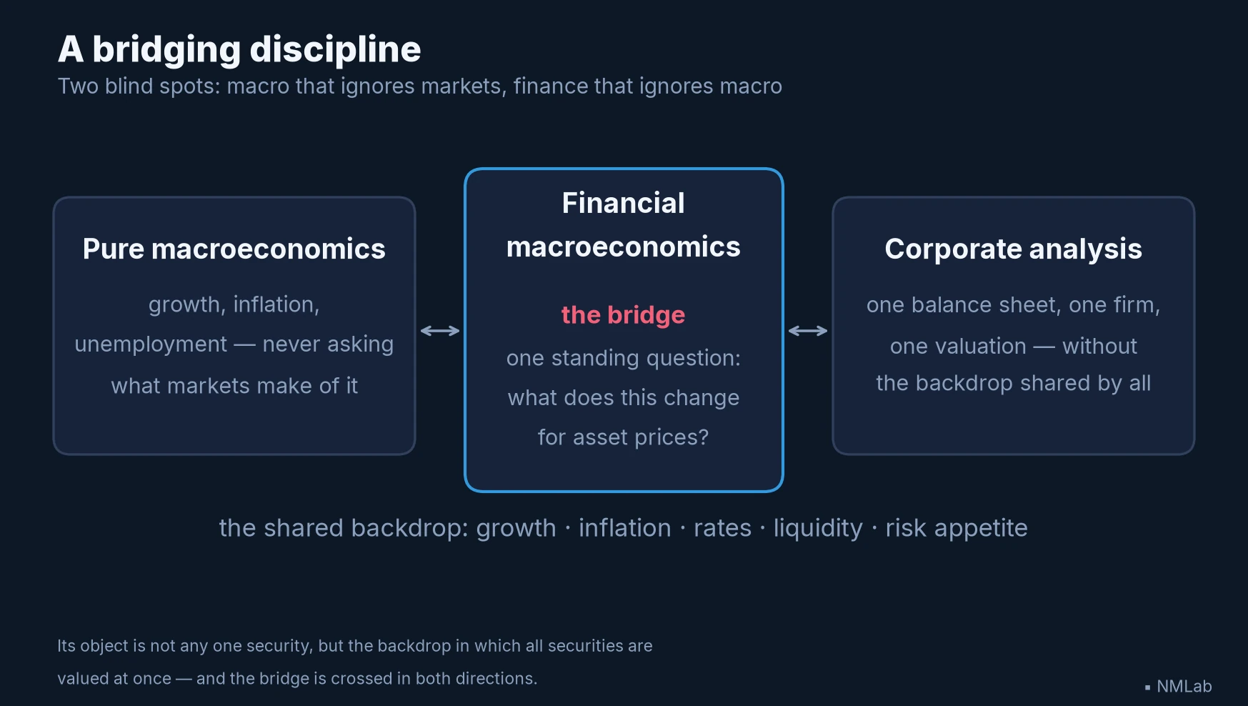
Of the three lenses, the figure shows only the two that financial macroeconomics directly bridges: pure macroeconomics and corporate analysis. The discipline connects the shared economic setting with the value of individual investments.

Why a single economic statistic can move markets

On the day it appears, a statistic does not pay anyone a cent: the payments already promised remain exactly what they were. What it moves lies elsewhere — expected profits, expected rates, expected risks, and therefore the price investors are willing to pay today.

Would you rather receive €100 today or €100 in one year? If an investment considered equally safe earns 4% a year, about €96 invested today will grow to €100 in one year.

Converting a future sum into today's value is called discounting. A future sum is generally worth less because today's money can already be used or invested, inflation can erode its purchasing power, and the promised payment may not arrive.

The required return, also called the discount rate, is the annual percentage an investor wants in exchange for waiting and bearing that risk; it bundles three building blocks — a real rate (the return on a safe investment, inflation stripped out), expected inflation, and a risk premium: the extra return demanded for accepting that those future payments are uncertain — that a promised payment may not arrive, or that a hoped-for profit may fall short. In this one-year example, dividing €100 by 1.04 gives about €96.15.

At 8%, the same promise of €100 in one year is worth only about €93, compared with about €96 at 4%: the final payment is unchanged; only the required return has increased. For the same future payment, required return and current price move in opposite directions.

The effect grows with time because the return compounds year after year. A promise of €100 in thirty years is worth about €31 at a 4% required return, but only €10 at 8%. This is why assets whose income lies far in the future react strongly to small changes in rates.

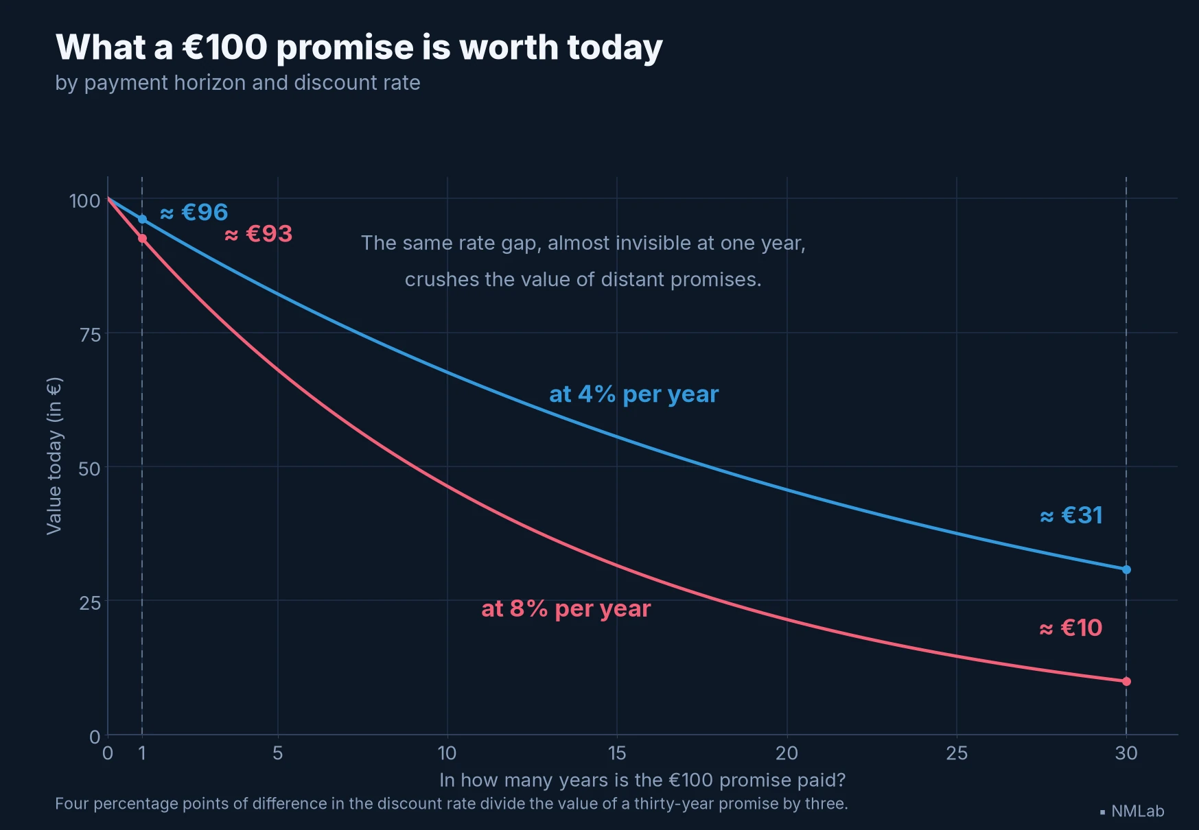
Moving from 4% to 8% takes a little over €3 off a one-year promise, but nearly €21 off the same promise thirty years out.

Here is a security that promises 0% and pays something all the same. When it is first issued, a bond allows a government or company to borrow: the initial investor lends money in exchange for promised payments, and the bond can later be sold to another investor.

Three terms are enough to follow the example: the coupon is the interest that may be paid over the life of the loan, the maturity date the date of final repayment, and the face value the amount repaid on that date. For the rest of the vocabulary, see The essential vocabulary of financial macroeconomics, without the jargon.

An OAT — short for the French obligation assimilable du Trésor — is a bond issued by the French government, and its price, like that of other bonds, is quoted as a percentage of face value rather than as a euro amount per security. The 0% May 2032 OAT is a particularly clear example because it pays no coupon and makes only one payment: €100 of face value on May 25, 2032.

At the February 3, 2022 auction — the sale organized by the government and settled on February 7 — its weighted-average price was €95.49 for €100 of face value. For an investor holding it to maturity, the sequence was concrete: pay €95.49 on February 7, 2022, receive nothing until May 25, 2032, then receive €100 — provided the government repaid as promised, and with the option of selling earlier at a price that might be higher or lower.

The “0%” refers to the coupon, not the investor's yield. Paying €95.49 and later receiving €100 means a total gain of €4.51 over about 10.29 years. That corresponds to an annualized yield of 0.45%, before fees and taxes.

$$\large \rule{0pt}{1.6em} P = \frac{100}{(1+0.0045)^{10.29}} \approx 95.49$$

The result, €95.49, matches the weighted-average price of the auction. The denominator reverses the accumulation of the 0.45% annual yield over 10.29 years: instead of moving €95.49 forward to 2032, it brings €100 backward to 2022. The match is close but not exact to the cent: 0.45% is itself a rounded figure, and Agence France Trésor publishes a weighted-average price and a weighted-average yield separately.

That OAT makes only one payment. Other bonds pay coupons, while some stocks pay dividends. Each future payment is called a cash flow.

You can skip the following formula on a first reading. The essential idea is to convert each payment into today's value and then add the results:

$$\large \rule{0pt}{1.6em} P \approx \sum_{t=1}^{T} \frac{\text{Expected cash flow}_t}{(1+r_t)^t}$$

The $\sum$ sign, read “sum,” means repeating the calculation for each payment, from the first, $t=1$, to the last, $T$, and adding the results. For a bond, $T$ is the maturity date; a stock has none, so the sum either runs on without end or stops at a horizon you choose, with an estimated resale value added on that date. The subscript on $r_t$ is a reminder that the required return may differ depending on how far off the cash flow is. For the 0% OAT there is a single €100 cash flow, so the general formula reduces to the calculation above; with a coupon-paying bond, the same operation would be repeated for every coupon.

The price ultimately depends on two forces pulling in opposite directions, set out like the top and bottom of a fraction: above, higher expected future payments — their amount and their timing — support the price; below, a higher required return — the compensation demanded for waiting and bearing risk — reduces it.

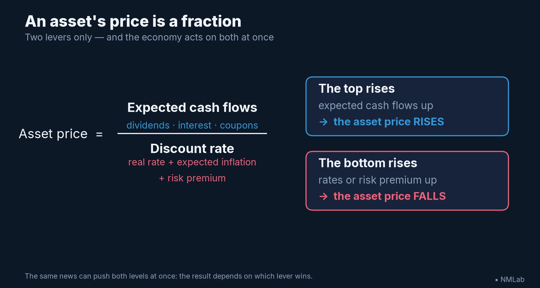
The fraction is a memory aid: each payment is actually discounted separately. As noted earlier, the discount rate brings together the real rate, expected inflation and the risk premium — three building blocks the journey returns to one by one.

A statistic can affect both forces. Strong economic activity may improve expected profits while also increasing inflation fears and expected interest rates; it also moves the risk premium investors demand — and it moves it more for a shaky company than for a solid one. The same news can therefore create opposing forces, which is why the market's response is never entirely automatic.

Why assets do not all react in the same way

The same shock comes in through different doors. A bond's payments are contractual; a company's profits move with activity; a currency can only be judged against another currency.

Take those doors in order. When rates rise — meaning that buyers require a higher market yield on comparable bonds — an older fixed-rate bond cannot raise its coupon, unlike a floating-rate note whose coupon resets with the market: its price is the only thing left to adjust, and it falls. Its promised payments cannot change, so the only way for it to compete with a newer bond is to cost less today: paying less for the same €100 at maturity raises the gain collected at repayment. The reverse happens when market yields fall. An inflation-linked bond is no exception: its payments track prices, not the required return. A central bank's policy rate — the rate, or range of rates, it sets or targets for overnight lending between banks — can influence market yields, but it is not the same rate.

Time matters. Modified duration estimates how much a bond's price changes for a small change in its yield. A modified duration of 5 means that a one-percentage-point rise in yield — for example, from 2% to 3% — would lower the price by about 5%, if everything else remained unchanged.

Modified duration takes the timing of every payment into account, not only the maturity date. It is close to the remaining life of a zero-coupon bond, but generally shorter when coupons pay back part of the money before maturity.

$$\large \rule{0pt}{1.6em} \frac{\Delta P}{P} \approx -D_{\mathrm{mod}} \times \Delta y$$

The Greek letter $\Delta$, “delta,” means “the change from before to after.” A one-percentage-point rise in the yield is written $\Delta y = 0.01$. For example, if a price moves from €100 to €95, then $\frac{\Delta P}{P}=-0.05$, or a 5% decline. The relationship remains an approximation and works best for small yield changes. It estimates the effect of yield alone, holding the promised payments and other market conditions unchanged.

Take our 0% May 2032 OAT again, this time looking at rates. At the February 3 auction, settled February 7, its price was €95.49 and its yield 0.45%; at the March 3 auction, settled March 7, its price was €94.84 and its yield 0.52%. That increase came even though neither the Federal Reserve nor the European Central Bank had raised its policy rate yet, and even though the invasion of Ukraine on February 24 had meanwhile brought buyers back into government bonds: the expectation of tightening was already pushing yields up, before any decision had been taken.

The yield therefore rose by 0.07 percentage point. In decimal form, the change is $0.0052-0.0045=0.0007$.

Because the bond makes no payment before maturity, its modified duration was close to 10.2 — its remaining life, 10.29 years, divided by 1 + 0.45%. The formula gives:

$$\large \rule{0pt}{1.6em} \begin{aligned} \text{Estimated change} &\approx -10.2 \times 0.0007 = -0.00714 \approx -0.71\% \\ \text{Observed change} &= \frac{94.84-95.49}{95.49} \approx -0.0068 \approx -0.68\% \end{aligned}$$

The estimated decline of 0.71% is close to the observed decline of 0.68%, so the actual case confirms the order of magnitude given by the formula.

Twenty-eight days separate the settlement dates. With an unchanged positive yield, moving closer to the repayment at par would have pushed the price slightly higher, offsetting a small part of the decline. The data come from the official OAT page and the March 2022 auction.

A stock, by contrast, promises nothing: its future cash flows are neither fixed nor guaranteed. Faster activity can lift sales and expected profits, and so support the price; but if it also fuels inflation and pushes rates up, those same profits are discounted at a higher required return, which weighs on their present value.

The net effect depends on the business model. A bank may, depending on the context, benefit from a wider gap between what it charges on loans and what it pays on funding; a heavily indebted company suffers more from costlier credit; a company whose value rests mainly on distant profits is generally more sensitive to rates.

That leaves the last door. A currency is never quoted on its own: the euro trades against the dollar, so its price depends on the relative prospects of two economies.

Higher expected rates in one currency area can attract capital and support that currency. But the link is not mechanical: relative growth, inflation, the credibility of the central bank, the external balance — the country's trade position with the rest of the world — and the flight to safety all count as well. A stronger home currency also reduces the value of the income an investor earns abroad.

The U.S. monetary tightening pushed the same shock through all three doors at once. The Federal Reserve began raising its main policy rate in March 2022 to fight inflation: its target range went from 0–0.25% before that first hike to 4.25–4.50% in December, and then to 5.25–5.50% in July 2023 (official history).

That shock pushed bond yields up and weighed particularly heavily on long-dated bonds and on stocks whose profits lay far in the future; on the currency market, expected rate differentials altered the relative appeal of the dollar. One environment, then, but as many reactions as there are combinations of expected cash flows, rates, and risk premiums.

Where did the movement actually land? The yield curve compares the yields required to lend to the government for different lengths of time — for example, two, ten, or thirty years — and shows whether an increase affects mainly short-term borrowing, long-term borrowing, or the whole market.

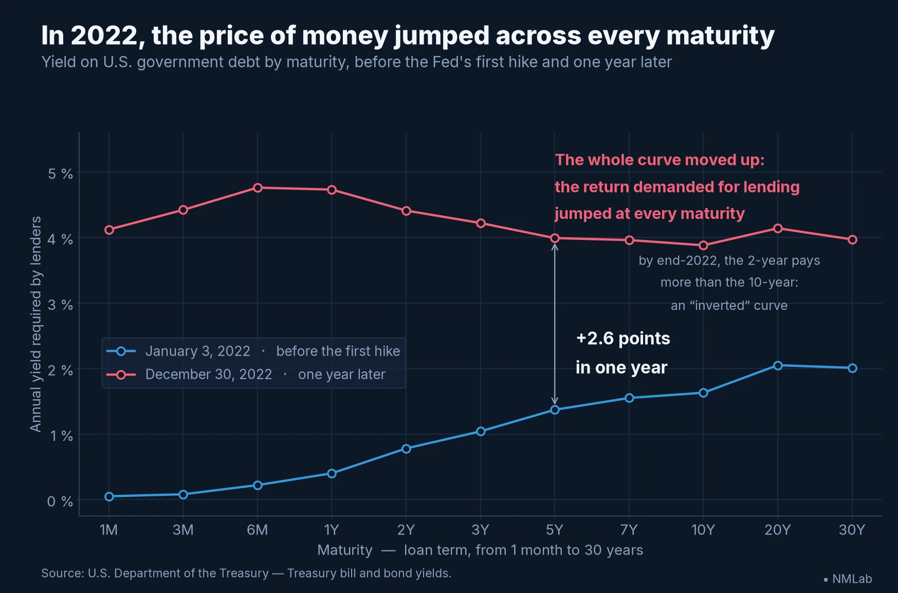
The entire curve moved higher in 2022. At year-end, the two-year yield exceeded the ten-year yield: that inversion was consistent with expectations of lower short-term rates ahead, often associated with a slowdown. It did not guarantee one, because long-term yields also embed a term premium — the extra yield demanded for lending long.

The market reacts to the gap, not the level

A company can report strong profits and watch its stock fall; a mediocre figure can lift the whole market. The absurdity is only apparent: prices already reflect expectations, so they respond mainly to the part of the news that was not anticipated. The first fell short of a bigger hope; the second was less bad than feared.

The consensus is the mean or median of a sample of forecasts collected before a release. It is a reference point, not a complete picture of expectations: it shows neither every scenario investors considered nor how much money was positioned for each one. Details within the release, revisions to earlier data, and accompanying comments can therefore still surprise. For an explanation of how macroeconomic data are produced, see Where do macro numbers come from?.

News that matches expectations often changes prices very little; on the measurement of these reactions, see research by the Federal Reserve. It can still move prices, though, if the survey consensus differs from the expectations actually embedded in prices — or if many investors have already bought and are taking their profits.

The surprise is not confined to a single number. Whether an inflation release surprises or the central bank decides nothing that day, the expected path of its policy rate over the coming months and years can move all the same. Prices in interest-rate markets let you estimate that path — an estimate that nevertheless contains risk premiums and does not reveal every investor's exact view, so it is not a sure forecast.

The news may also change expected profits or investors' willingness to bear risk. The central bank itself also watches financial conditions — the cost and availability of credit, asset prices, exchange rates and funding stress, taken together. Markets try to anticipate its decisions while it monitors their reaction.

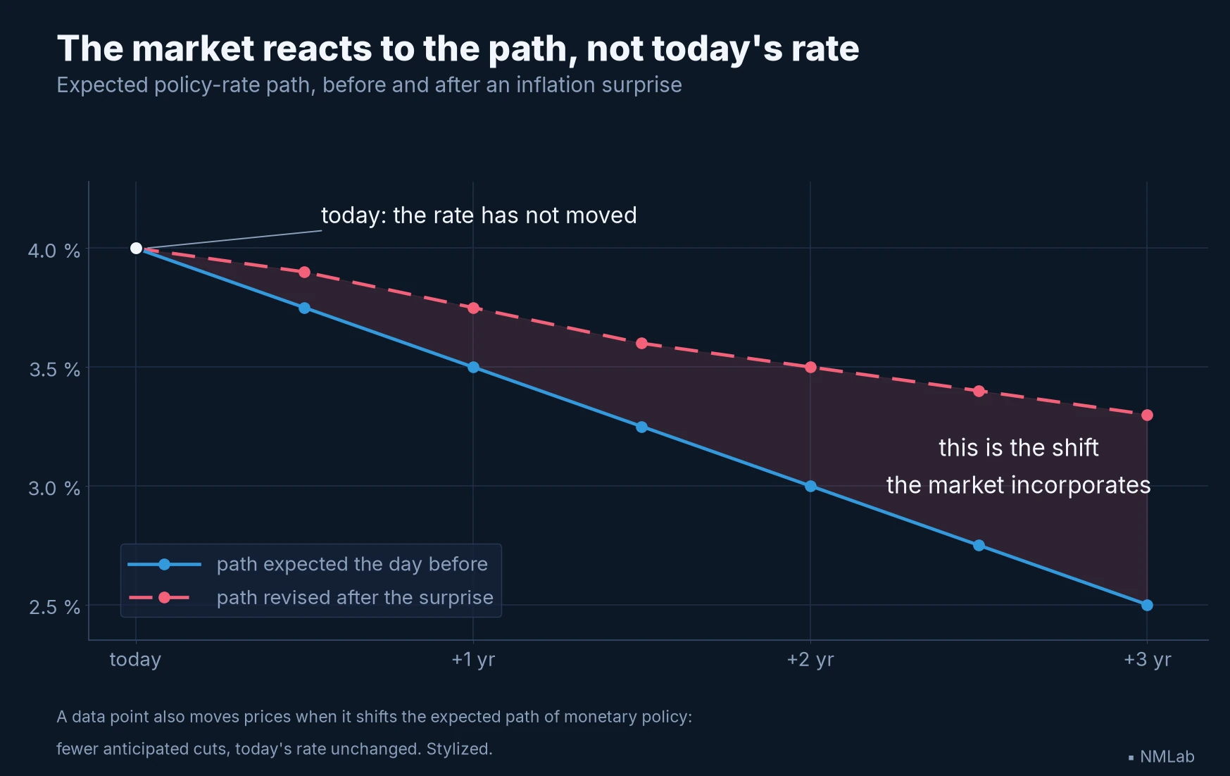
Stylized example: what the surprise moved is the years ahead, not today's rate.

In late 2023, investors firmed up their expectations of rate cuts before any were decided. Long-term yields fell, stocks rose and financial conditions eased; those moves, however, also reflected falling inflation, shifts in the term premium and in risk appetite. Monetary-policy expectations were therefore already at work, without explaining everything (Federal Reserve report).

The mirror acts on what it reflects

An ordinary mirror changes nothing about what it shows; this one does. Markets do not merely reflect the economy: they change it in turn, through three main channels. Wealth first: a lasting rise in the stock market or in real estate can encourage the households that own those assets to spend, and a fall can make them more cautious. Credit next: when interest rates and the premiums required by lenders rise, households and businesses borrow less, and purchases and investment projects are put off. Exchange rates last: a stronger currency makes imports cheaper but can hurt exporters, while a weaker currency generally has the opposite effect.

Wealth, credit, exchange rates: these are the three channels through which financial conditions reach the economy. When those conditions tighten, financing a project generally becomes harder; when they ease, financing becomes more accessible.

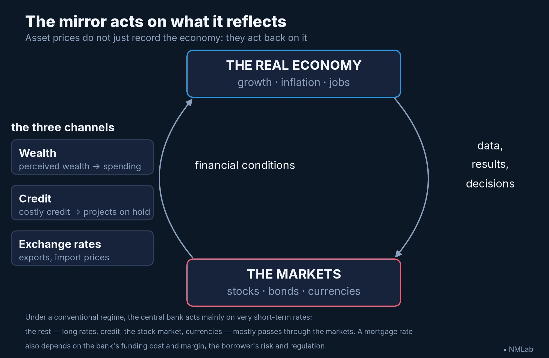
The loop has no starting point: the conditions sent back become the economy the next release will measure.

Under a conventional regime, a central bank mainly steers very short-term rates, through one or more policy rates, and communicates about what it might do next. It can also act through liquidity and through its balance sheet, which carries the portfolio of securities it holds; it is the markets that transmit those impulses to long-term borrowing costs, asset prices, and currencies.

Transmission is not mechanical. A mortgage rate also depends on a bank's funding cost and margin, the borrower's risk, regulation, and sometimes public guarantees. The central bank provides the impulse; the financial system determines its strength and reach.

What macro can — and cannot — do

Let us say it plainly: understanding these mechanisms does not let you predict every market move. Known information is generally already reflected in prices.

No regularity is immune to its context. In 2022, higher inflation and interest rates drove both stocks and bonds lower, weakening the usual diversification between the two. An inverted yield curve is often associated with a future recession — as officially dated by the National Bureau of Economic Research (NBER) — but it neither guarantees one nor sets its date: the inversion that began in July 2022, one of the longest on record, was not followed by the recession that was expected.

A market regularity is not a law of nature. A planet does not leave its orbit because someone has published the law that describes it; a market, by contrast, can change its behavior as soon as participants identify and exploit a pattern. Arbitrage — in the broad sense, the capital that moves into the gap a pattern leaves open — then tends to close it. A second mechanism, reflexivity, appears when expectations change the very reality they seek to predict. Together, these two effects make it difficult to keep choosing the best times to buy and sell, a practice known as market timing. Being right about the economy is not always enough: the scenario may already be priced in, the timing may not match, or another force may dominate.

What is left, then? A great deal. Financial macroeconomics remains useful for recognizing the dominant regime: high or low inflation, rising or falling rates, expansion or slowdown. These regimes guarantee no return, but they change the risks a portfolio faces. The discipline also helps distinguish a genuine surprise from information that was already expected.

Above all, it helps identify risks and avoid decisions made in panic or euphoria. Over a long savings horizon, that behavioral discipline can matter more than one successful forecast.

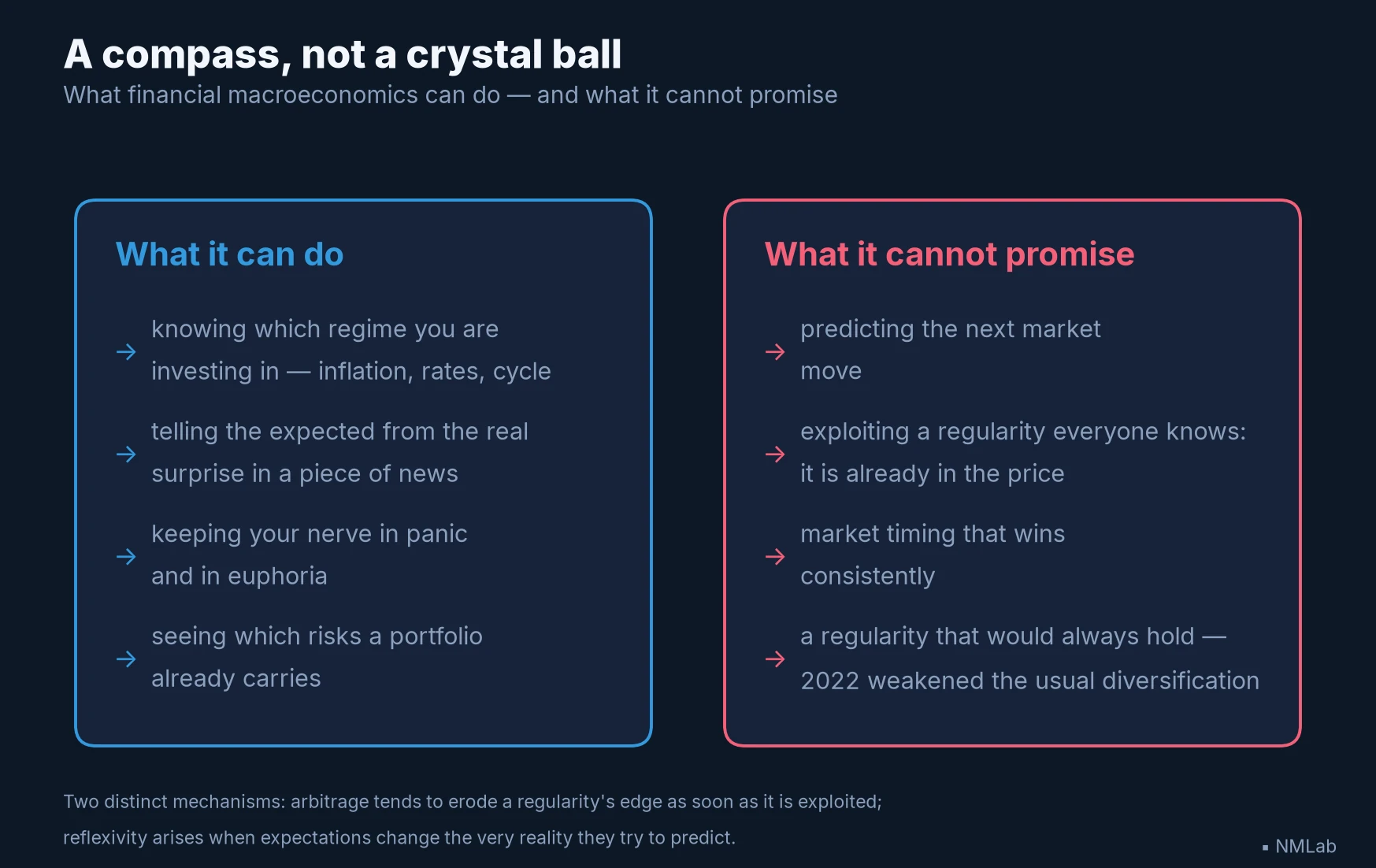
The right-hand column is not a list of failures: it is what no reading of the economy can buy.

The roadmap

The next modules will take up each idea in turn. A word on the difficulty curve: this journey starts assuming nothing and ends demanding something — the later chapters ask you to read data series, orders of magnitude and, occasionally, a correlation. Every chapter therefore states its level and its prerequisites in an opening box.

Four stages:

1. The basics: gross domestic product, money, inflation, and interest rates.
2. Economic dynamics: the business cycle, employment, indicators, and central banks. The big macro variables that move your investments provides an initial overview.
3. Policies and markets: monetary policy, fiscal policy and public debt, global liquidity, credit and crises, and investment regimes.
4. Practice: the analyst's dashboard and the closing synthesis.

There is no need to wait for the end: a macro monitoring routine is enough to start following the economy from this module on.

The thread running through the journey goes from the pandemic to the slowdown in inflation and the debate over a soft landing in 2024–2025. From COVID to the soft landing provides the map.

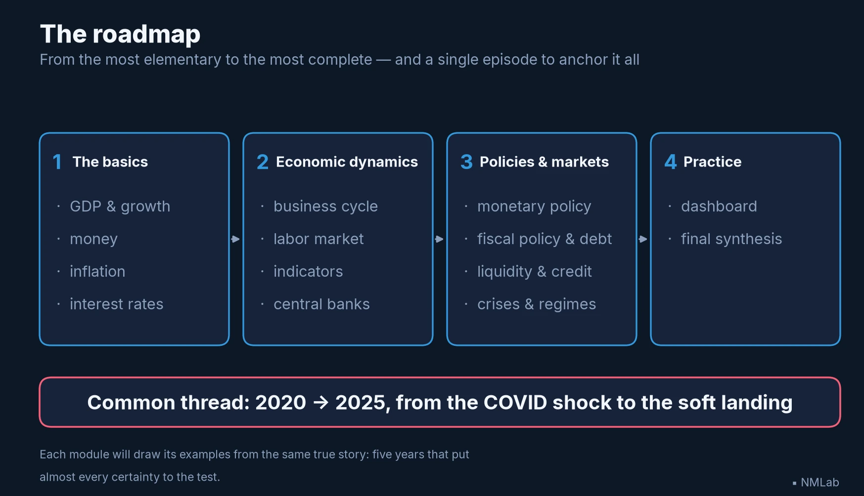
Each stage assumes the one before it; the 2020-2025 thread runs through all four.

Key takeaway

• A bridging discipline — The economy moves at the pace of quarters; markets reprice by the second. Financial macroeconomics connects the two by studying the common setting — growth, inflation, rates, liquidity, appetite for risk — in which every investment is valued. A price is an observable fact, not a truth about value: an opinion about the future.
• Discounting links the future to today's price — Expected future cash flows on top, the required return underneath, its weight growing with every year of waiting. A statistic pays nobody a cent: it moves one, the other, or both, sometimes in opposite directions.
• One shock, three doors — Contractual payments for the bond, uncertain profits for the stock, the relative prospects of two economies for the currency; the distance of the income and the risk premium do the rest. The setting is shared, the reaction is not.
• The market reacts to the gap, not the level — Expectations are already in the price; what moves it is mainly the part of the news that was not anticipated. Hence the good figures that sometimes send a stock down, and the bad ones that send it up.
• The mirror acts on what it reflects — Wealth, credit, exchange rates: when financial conditions tighten, financing a project generally becomes harder; when they ease, easier. Prices do not merely read the economy; they move it in turn.
• A compass, not a crystal ball — Recognizing the dominant regime, telling a genuine surprise from news that was already expected, seeing which risks a portfolio carries: that is a great deal, and it is not a forecast. The discipline says what world you are investing in, not what will rise tomorrow.

The rest of the journey

One objection is still hanging in the air: if everything you can learn about the economy is already in prices, why learn it? The next chapter answers it by turning that first intuition on its head — not to guess the next number, but to know what world you are investing in and which risks you are carrying. Next chapter: “Why investors need to understand the economy”. Until then, keep the intuition this chapter leaves you with: understanding the economy does not tell you what markets will do; it tells you what they react to — and that is already a great deal.

Sources and references

• Bureau of Labor Statistics, Employment Situation and release calendar.
• U.S. Securities and Exchange Commission (Investor.gov), what a stock is and what shareholders are entitled to.
• Agence France Trésor, 0% May 2032 OAT page, February 2022 auction, and March 2022 auction.
• Federal Reserve, federal funds rate history, monetary policy tools, research on stock-market reactions to macroeconomic news and the Monetary Policy Report of March 2024.
• European Central Bank, key ECB interest rates and open market operations, liquidity and asset purchases.
• U.S. Treasury, daily yield-curve data for 2022.
• Federal Reserve Bank of St. Louis (FRED), 10-year minus 2-year Treasury spread — length of the 2022-2024 inversion.
• Federal Reserve Bank of New York, expectations, the term premium and recession signals.
• Federal Reserve, FCI-G financial-conditions index.
• National Bureau of Economic Research (NBER), U.S. business-cycle dating.
• John Maynard Keynes, The General Theory of Employment, Interest and Money (1936) — expectations and investment.
• Milton Friedman and Anna J. Schwartz, A Monetary History of the United States, 1867–1960 (1963).
• Robert E. Lucas Jr., “Econometric Policy Evaluation: A Critique” (1976).
• Eugene F. Fama, “Efficient Capital Markets: A Review of Theory and Empirical Work”, Journal of Finance (1970).
• John Burr Williams, The Theory of Investment Value (1938) — discounting future cash flows.
• Frederick R. Macaulay, Some Theoretical Problems Suggested by the Movements of Interest Rates, Bond Yields and Stock Prices in the United States since 1856 (1938).
• George Soros, The Alchemy of Finance (1987) — reflexivity.