26. The Quantity Theory of Money (MV = PQ): Linking Money, Prices and Activity

In 1568, a jurist from Anjou named Jean Bodin publishes a short reply to a senior official of the mint, one Sieur de Malestroit. The debate turns on a riddle of the century: for decades, in France as across Europe, prices have risen without pause. Malestroit holds a reassuring explanation: the rise is merely an accounting illusion, born of the debasement of coins whose metal kings have clipped. Bodin sweeps the argument aside and names the true culprit, to be sought beyond the seas: gold and silver, landed by the galleon-load from the mines of the Americas — those of Potosí above all — flood the Old Continent and drive up the price of everything. "The principal cause that raises the price of everything, in whatever place it be," he writes, "is the abundance of that which gives things their valuation and price."

Bodin was not the first: Copernicus had sensed it as early as 1526 — "money loses its value most of all through excessive abundance" — and the Spanish theologian Martín de Azpilcueta had stated it in 1556. But Bodin gave the most resounding demonstration, and history has kept his name. One point, though, that the textbooks forget: this "price revolution" was slow. Over a century and a half, European prices were multiplied by three to six depending on the region — barely 1% a year. Nothing like a blaze: a rising tide, imperceptible from one year to the next, irresistible over a lifetime.

Four centuries later, Bodin's intuition has an equation. It fits in four letters, MV = PQ, and claims to link, in a single stroke, the quantity of money, prices and activity. It is one of the most famous relations in economics — and one of the most misleading, because it is at once always true and often useless. To dismantle that paradox is to understand why money matters, when it matters, and when it says nothing.

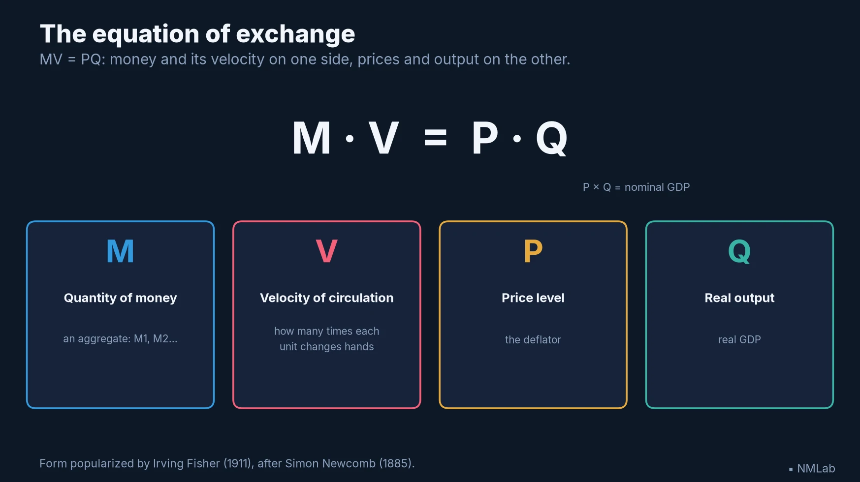
Four letters to link money to the economy: the quantity of money and its velocity on one side, prices and output on the other.

At a glance — Level: Intermediate · Prerequisites: chapter 24 and chapter 25

By the end of this chapter, you will be able to:

• explain why MV = PQ is always true — and why that is precisely what makes it silent on its own;
• name the three assumptions that turn the identity into a theory, and which one gives way;
• see why the money-price link sleeps in calm regimes and wakes in feverish ones.

The equation that cannot be false

Let us read its four terms. Three are old acquaintances: M, the quantity of money — one of the previous chapter's aggregates; P, the general price level; Q, real output, the volume of goods and services, the real GDP of chapter 10. Multiply the last two: P × Q is nominal GDP. That leaves V, the velocity of circulation: the number of times a unit of money changes hands to buy that output over a year. If the money stock is 1,000 and $2,000 of GDP is bought, then each unit has served twice: V = 2.

$MV = PQ$

The original form is Irving Fisher's: 1911, The Purchasing Power of Money. He writes it with the volume of transactions rather than output, and loyally credits a predecessor, the astronomer and economist Simon Newcomb (1885). To no avail — as with Bodin, posterity has kept only one name, Fisher's, and the version just written.

And here is the trap, the one you must have grasped never to be caught out: this equation literally cannot be false. For velocity is never measured directly — no one tracks banknotes. It is defined as the ratio that makes the equality true: $V \equiv PQ / M$. Velocity is the residual, the number written in after the fact to balance the books. So MV = PQ is an accounting identity — true by construction, everywhere, always, like "bachelor = unmarried man." An equation that can never be disproved predicts nothing on its own: it organizes language, it does not say what causes what. The whole difficulty of the chapter lies there.

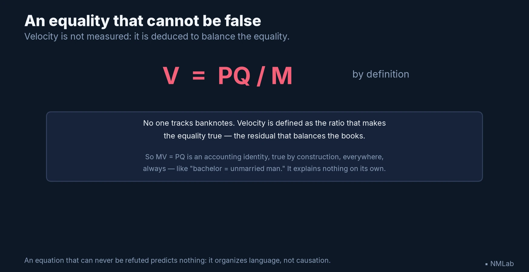
Velocity is not measured, it is deduced: V is the figure that balances the equality. Hence an identity always true — and mute on its own.

From identity to theory

How does a tautology become the quantity theory of money, the one that holds money governs prices? By adding three hypotheses — three locks that turn the inert equality into a chain of causation.

First lock: velocity is stable, or at least predictable. If V does not move, a change in M passes fully into the right-hand side. Second lock: real output Q is determined elsewhere — by labor, capital, technology — independently of the quantity of money, at least in the long run, when the economy runs near its capacity. Third lock: causation runs from money to prices, not the reverse. Tighten the three, and the result drops out: if V is fixed and Q given, then any rise in M spills entirely into P. Double the money, you double prices. That is the quantity theory in its pure form — and Bodin's intuition, at last formalized.

The Cambridge school takes the same idea by the other end — Alfred Marshall first, Arthur Pigou in 1917: no longer the money you spend, but the money you keep. People wish to hold a fraction k of their income in cash balances, so $M = k \cdot PQ$, where k is merely the inverse of velocity. The gaze shifts — you start from the demand for money — but the content is identical. Milton Friedman would carry the reversal through to the end in 1956: the quantity theory is not first a theory of prices, but a theory of the demand for money. Everything therefore rests on the soundness of the three locks. And the first, we shall see, is a lock of straw.

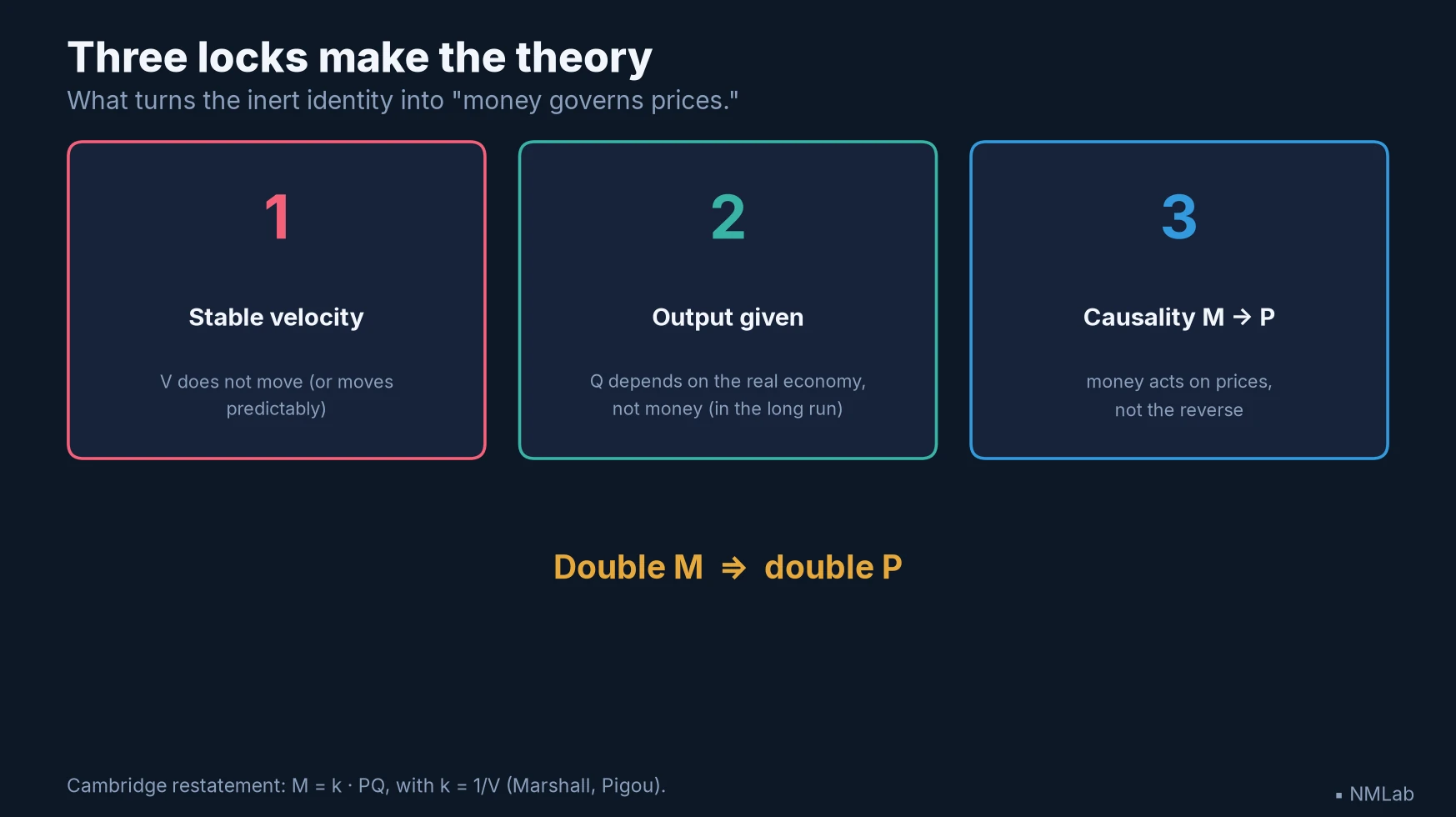
Three locks turn the identity into a theory: stable velocity, given output, causation money → prices. Double M, you double P.

From the slow tide to hyperinflations

Before sawing through the first lock, let us do the theory justice: the link between money and prices is neither a fantasy nor an iron law. It appears in full light in two situations — the very long run, and the extremes.

Over the very long run, money and prices do rise together: Bodin's price revolution was the first testimony, and American history confirms it in its own way. Since 1959, the M2 money stock of the United States has been multiplied by eighty, and the price level by eleven. The link is undeniable — but the ratio is not one-for-one, and therein lies the whole lesson: the gap is absorbed by the other two terms of the equation, real output, which has grown strongly (Q), and velocity, which has, for its part, fallen sharply (V). Money and prices march in the same direction, never at quite the same pace.

At the extremes, the demonstration turns brutal. In hyperinflations, the quantity of money explodes and prices follow at a gallop, so fast that the equation seems to become an iron law again. Germany in 1923: by November, it takes 4.2 trillion marks for a single dollar, and the state prints notes of a hundred trillion. Hungary in 1946, the worst episode ever measured: prices double on average every fifteen hours, a monthly rate on the order of 4 × 10¹⁶ percent. Zimbabwe in 2008. Phillip Cagan, who made the classic study of them in 1956, even offers a threshold: hyperinflation begins the month prices rise by more than 50%. And one spring makes it all worse: when money melts before one's eyes, no one wants to hold it any longer; each person spends it as fast as possible, so that velocity itself races and fuels prices further. M and V add up in the catastrophe.

It is this regularity at the extremes that licenses Milton Friedman's most famous formula: "Inflation is always and everywhere a monetary phenomenon in the sense that it is and can be produced only by a more rapid increase in the quantity of money than in output" — stated in 1970, and often quoted while forgetting the second half of the sentence, the most important part. For the nuance changes everything: Friedman speaks of persistent inflation, the kind that lasts, not of a one-off rise in oil or a supply bottleneck. The link holds over time and at high intensity; it dissolves in the quiet short run.

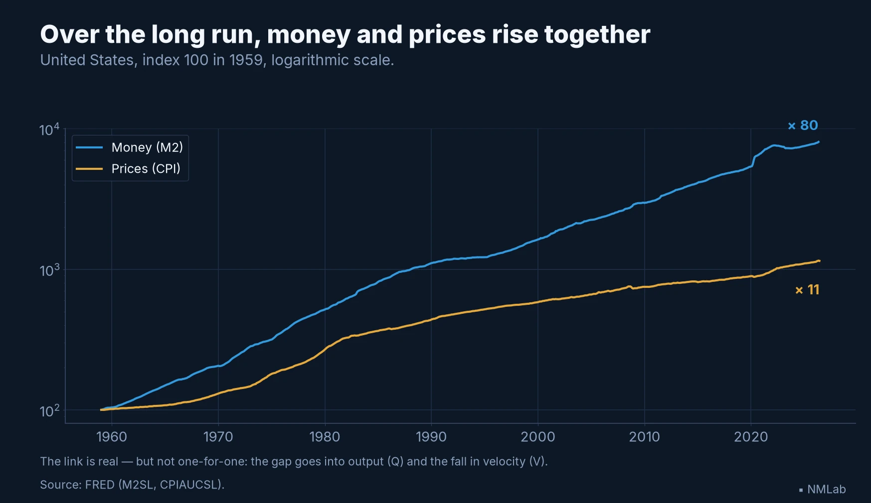
Over the long run, money and prices rise together — M2 by eighty, prices by eleven since 1959: the link is real, never one-for-one.

The weak link: velocity

Take the first lock again — "velocity is stable" — and look at the data. They break it cleanly. The velocity of M2 in the United States, far from a constant, has done the splits: around 1.8 in the postwar decades, a peak of 2.19 in 1997, then a long slide to a floor of 1.13 in the spring of 2020, before a partial rebound toward 1.4 in early 2026. In plain terms: at the trough of 2020, each dollar of M2 served only a little more than once a year to buy GDP, against more than twice in 1997. Velocity was nearly halved in a quarter-century.

Now a fall in V cancels, arithmetically, a rise in M. That is exactly what happened after 2008, as chapter 24 showed: the Federal Reserve inflated the base, but it stayed asleep in excess reserves; broad money — the M of our equation — grew only moderately, its velocity collapsing opposite, so that prices did not budge. The prophets of hyperinflation, transfixed by the swelling base, had confused central-bank money with the money that circulates — and forgotten the velocity sinking opposite. As long as velocity slips away like this, MV = PQ stays a true identity and a mute theory: nothing can be deduced from M without knowing what V does. This weak link is so central that it deserves its own chapter — the next one is devoted to it. For now, remember that velocity is the variable that decides whether money speaks or stays silent.

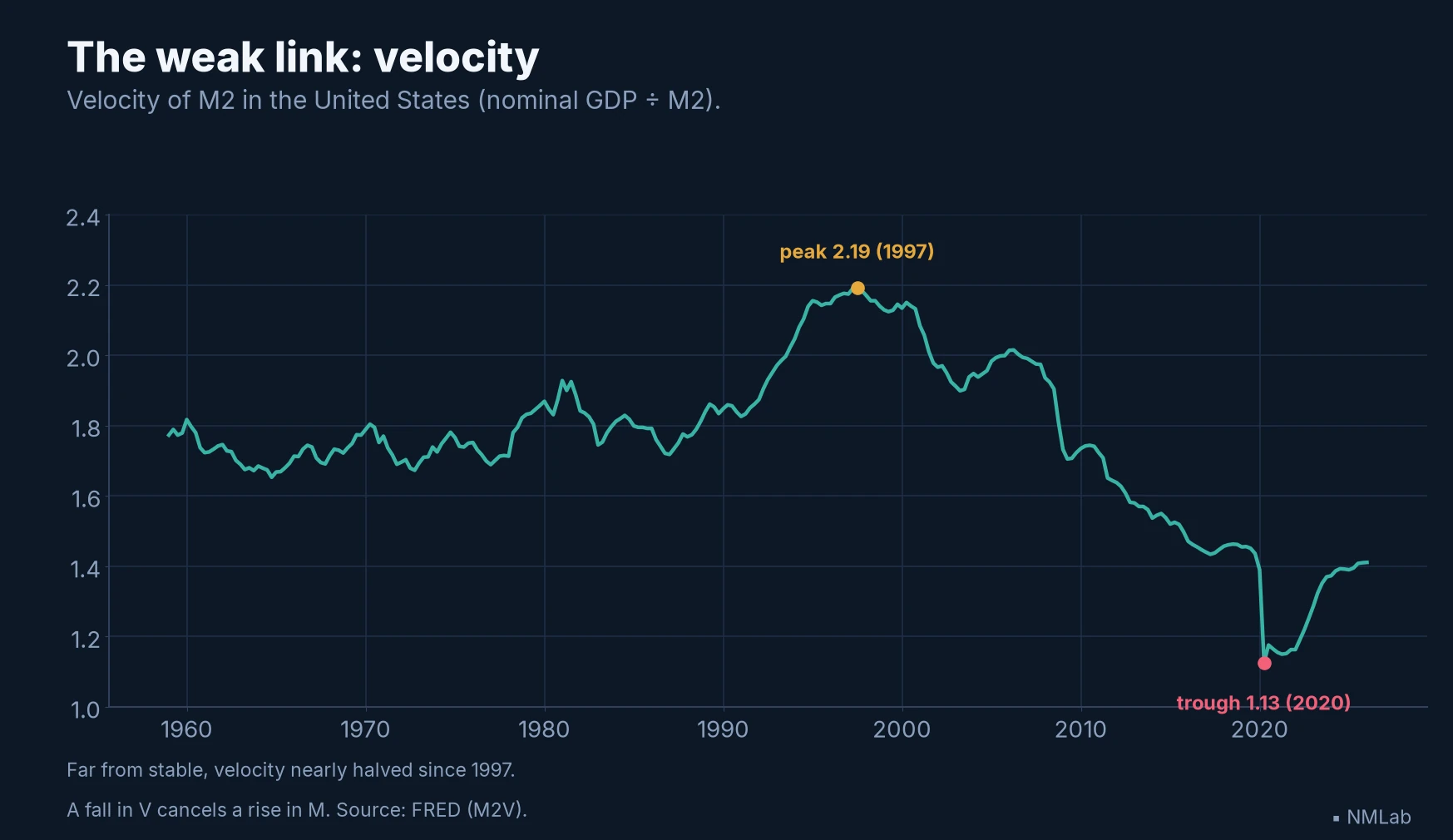
The lock of straw: far from stable, the velocity of M2 was nearly halved since 1997. A fall in V cancels a rise in M.

Monetarism and its defeat

If you believe in the three locks, a policy imposes itself: to master prices, it is enough to hold money on a tight rein. Such was the program of monetarism, and it had its hour of glory. On 6 October 1979, Paul Volcker, freshly appointed to head the Fed, announces a change of method: the central bank will henceforth target the quantity of reserves to curb the growth of M1 and M2. Interest rates soar — to nearly 20% — a severe recession follows, but the great inflation of the 1970s is broken. The theory of Bodin and Friedman, applied, had worked.

And yet the Fed abandons money targeting as early as the autumn of 1982. Why give up a tool that had just won? Because the velocity lock had failed mid-maneuver: the arrival of new interest-bearing account types and the instability of the demand for money made M1 unreadable — its relation to prices slipping away just as it was being used as a compass. Margaret Thatcher's United Kingdom met the same setback: its 1980 financial strategy set multi-year targets for the £M3 aggregate, systematically overshot. Behind these two failures, one and the same mechanism: Goodhart's law from chapter 6, at work at full scale — the regularity unravelled at the very moment it was being used as a compass. Monetarism won a battle, the disinflation of the 1980s, and lost the war of instruments: no major central bank today steers the quantity of money. All steer its price, the interest rate — as chapter 24 established.

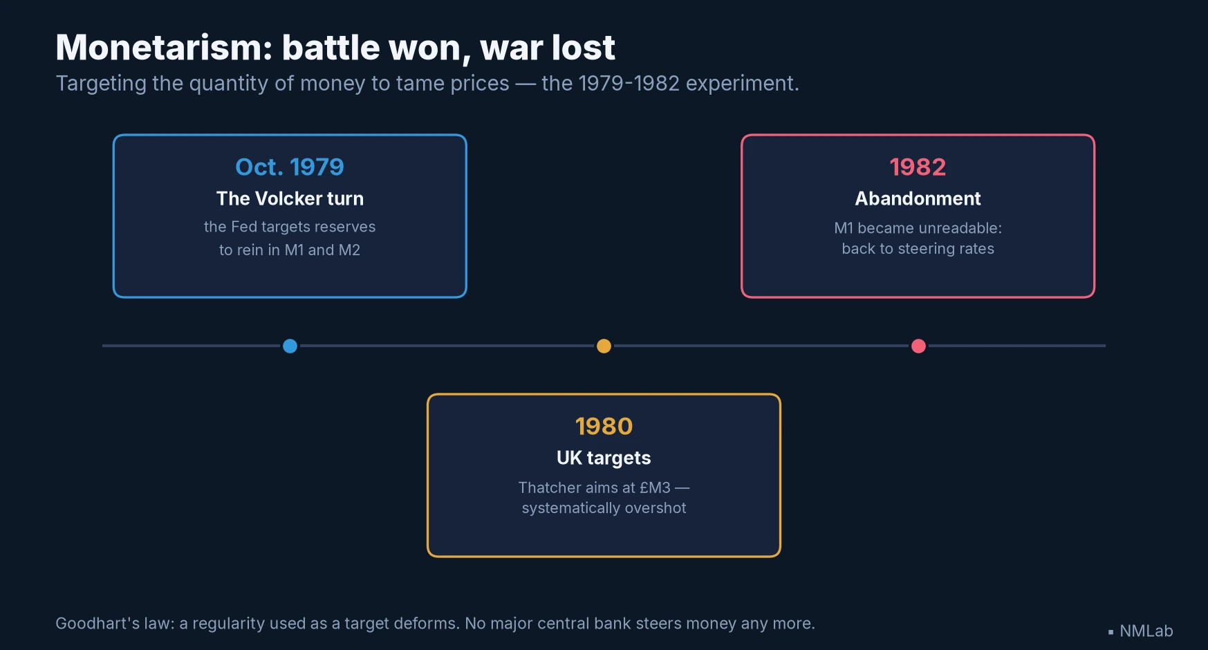
Monetarism won the disinflation and lost the instruments: targeted, the aggregate slipped away (Goodhart's law). What remains is steering by rates.

When the equation speaks again: 2020-2022

The story could have stopped there — equation true but useless, monetarism buried. Then came 2020, and the counter-test that chapter 24 laid out: broad money deposited straight into households' accounts, spent, and inflation cresting sixteen months after it. Reread the episode with our four letters and it loses its mystery. M leaps; Q, hemmed in by shortages and saturated capacity, cannot absorb the shock; and V, instead of cushioning as it had for twenty years, stops falling and then climbs — people spend the money they receive instead of letting it sleep. Three terms pushing the same way: only P is left to balance the equality.

Hence the lesson the Bank for International Settlements draws in early 2023: the strength of the link between money growth and inflation depends on the regime — "one-to-one when inflation is high, virtually non-existent when it is low." That reconciles everything. The three locks hold only under high pressure: when inflation sleeps and expectations are anchored, velocity absorbs the jolts of money and the M → P link stretches until it vanishes; when inflation awakens, velocity stops cushioning, and the equation becomes binding again. It is therefore not the identity MV = PQ that is conditional — it stays true by construction, always — but the quantity theory, the causal link from money to prices: that sleeps in calm regimes and wakes in hot ones, exactly the reverse of the moment it is usually invoked.

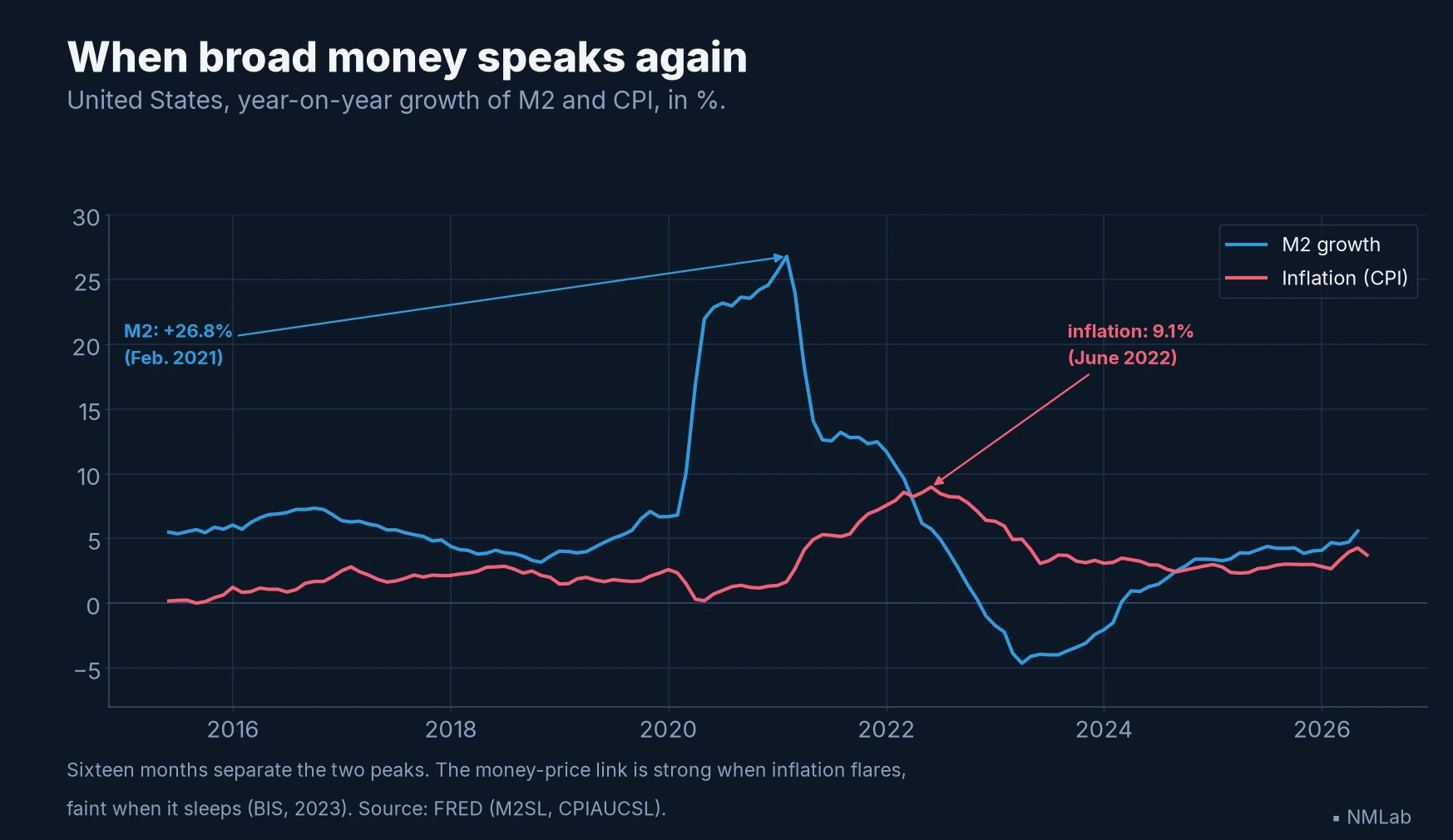
Broad money led inflation by sixteen months. The link is not mechanical — it is regime-conditional: strong when inflation flares, faint when it sleeps.

What it changes for your investments

The equation of exchange is not a crystal ball; it is a diagnostic grid. Its virtue is to force the right question: when money accelerates, where does it go? Three possible destinations, one equation to hold them. New money can pour into prices (P) — the nightmare of 2021-2022. It can fund a rise in output (Q) — the dream, when idle capacity waits. Or it can be swallowed by a fall in velocity (V) — the purgatory of 2008-2014, when the money created simply sat still. Faced with any money surge, break it down: through which of the three channels will it pass?

From there, three reflexes. Never reason on M alone: a quantity of money without its velocity says nothing, and confusing the two was the error of the hyperinflation prophets of 2010. Look at the regime before the aggregate: at low, anchored inflation, a monetary acceleration is a faint signal; when inflation takes off and the economy saturates, ignoring it costs dearly. Finally, translate the signal into portfolio risk: strong, lasting money growth, in an economy near its limits, heralds price pressures — and therefore, sooner or later, a rise in rates, the most direct and mechanical channel to the value of your bonds, met in chapter 4. The equation will never tell you what to buy tomorrow; it tells you which monetary regime you are investing in, and which of the three channels to watch.

Key takeaway

• The equation — MV = PQ, form due to Fisher (1911), after Newcomb (1885): the quantity of money (M) times its velocity of circulation (V) equals nominal GDP — prices (P) times real output (Q). A multiplication, nothing more.
• An identity, not a prediction — Since velocity is defined as PQ/M, the equality is true by construction, always. It predicts nothing on its own.
• Three locks — It becomes a theory (money governs prices) under three hypotheses: stable V, Q set by the real economy, causation M → P. Cambridge restatement: M = k·PQ, with k = 1/V (Marshall, Pigou).
• The link is real at the extremes — Long run (U.S. M2 ×80, prices ×11 since 1959) and hyperinflations (Weimar, Hungary 1946), where M and V race. Friedman: persistent inflation "is always and everywhere a monetary phenomenon."
• The weak link: velocity — Far from stable, V was nearly halved since 1997 (2.19 → 1.13 in 2020). A fall in V cancels a rise in M: the money of 2008-2014 slept.
• Target yesterday, thermometer today — Money targeting (Volcker 1979, British £M3): disinflation won, tool abandoned by 1982 (Goodhart's law) — central banks steer the price, not the quantity. But the money-price link remains regime-conditional (BIS 2023): faint when inflation sleeps, strong when it flares. The equation wakes in the fever.

The rest of the journey

The equation of exchange has led us to a culprit and an innocent. The innocent is M: the quantity of money, on its own, does not predict prices. The culprit — or rather the key witness — is V, that velocity by turns stable, collapsed and reborn, which decides whether a rise in money ends up in prices or is lost in the sand. We have crossed its path at every turn of this chapter without ever really opening it up. It is time. Next chapter: "The Velocity of Money: Why It Matters." Until then, an exercise: take the M2 money stock and nominal GDP of the United States, divide the second by the first, and watch velocity plunge after 2008 — You will understand at a stroke why so much money did not make so much inflation.

Sources and further reading

• Jean Bodin, La Response … au paradoxe de M. de Malestroit touchant l'enchérissement de toutes choses, 1568 — the abundance of American metals as the cause of rising prices.
• Nicolaus Copernicus, Monetae cudendae ratio, 1526; Martín de Azpilcueta, Comentario resolutorio de cambios, 1556 — the statements of the quantity theory that predate Bodin.
• David Hume, "Of Money," in Political Discourses, 1752 — proportionality of money and prices, long-run neutrality.
• Earl J. Hamilton, American Treasure and the Price Revolution in Spain, 1501-1650, Harvard University Press, 1934 — the silver of Potosí and the measurement of the price revolution.
• Irving Fisher, The Purchasing Power of Money, Macmillan, 1911 — the equation of exchange (MV = PT), after Simon Newcomb, Principles of Political Economy, 1885.
• Arthur C. Pigou, "The Value of Money," Quarterly Journal of Economics, 1917; Alfred Marshall, Money, Credit and Commerce, 1923 — the Cambridge equation (M = kPY).
• Milton Friedman & Anna J. Schwartz, A Monetary History of the United States, 1867-1960, Princeton University Press, 1963; Milton Friedman, The Counter-Revolution in Monetary Theory, Institute of Economic Affairs, 1970 — "inflation is always and everywhere a monetary phenomenon…" (p. 24).
• Phillip Cagan, "The Monetary Dynamics of Hyperinflation," in M. Friedman (ed.), Studies in the Quantity Theory of Money, University of Chicago Press, 1956 — the 50%-a-month threshold.
• Steve H. Hanke & Alex K. F. Kwok, "On the Measurement of Zimbabwe's Hyperinflation," Cato Journal, 2009.
• Robert E. Lucas Jr., "Two Illustrations of the Quantity Theory of Money," American Economic Review 70(5), 1980, pp. 1005-1014 — money-price proportionality appears once the series are filtered of short-run fluctuations: the link is a long-run fact, not a quarterly one.
• Pedro Teles, Harald Uhlig & João Valle e Azevedo, "Is Quantity Theory Still Alive?", Journal of Money, Credit and Banking 48(5), 2016, pp. 875-895 — the relation holds in high-inflation countries and dissolves in low-inflation, well-anchored ones: the academic counterpart to the BIS result.
• Charles Goodhart, "Problems of Monetary Management: the U.K. Experience," 1975 — Goodhart's law.
• Federal Reserve, "The Reform of October 1979" — the Volcker turn and reserve targeting.
• Claudio Borio, Boris Hofmann & Egon Zakrajšek, "Does money growth help explain the recent inflation surge?", BIS Bulletin no. 67, 26 January 2023 — the regime-conditional money-inflation link.
• Figure data: FRED (M2SL, M2V, CPIAUCSL, GDP) — vintage of 24 July 2026.